Quantitative Analysis
Parallel Processing
Numerical Analysis
C++ Multithreading
Python for Excel
Python Utilities
Services
Author
Printable PDF file
I. Basic math.
II. Pricing and Hedging.
III. Explicit techniques.
IV. Data Analysis.
V. Implementation tools.
1. Finite differences.
2. Gauss-Hermite Integration.
3. Asymptotic expansions.
4. Monte-Carlo.
5. Convex Analysis.
A. Basic concepts of convex analysis.
B. Caratheodory's theorem.
C. Relative interior.
D. Recession cone.
E. Intersection of nested convex sets.
F. Preservation of closeness under linear transformation.
G. Weierstrass Theorem.
H. Local minima of convex function.
I. Projection on convex set.
J. Existence of solution of convex optimization problem.
K. Partial minimization of convex functions.
L. Hyperplanes and separation.
M. Nonvertical separation.
N. Minimal common and maximal crossing points.
O. Minimax theory.
P. Saddle point theory.
Q. Polar cones.
R. Polyhedral cones.
S. Extreme points.
T. Directional derivative and subdifferential.
U. Feasible direction cone, tangent cone and normal cone.
V. Optimality conditions.
W. Lagrange multipliers for equality constraints.
X. Fritz John optimality conditions.
Y. Pseudonormality.
Z. Lagrangian duality.
[. Conjugate duality.
VI. Basic Math II.
VII. Implementation tools II.
VIII. Bibliography
Notation. Index. Contents.

Pseudonormality.


e use the notation of the problem ( Smooth optimization problem ).

Definition

(Pseudonormality). The vector $x^{\ast}\in C$ is called "pseudonormal" if one cannot find the vectors $\lambda$ , $\mu$ and a sequence MATH such that

1. MATH ,

2. $\mu\geq0$ , MATH and MATH .

3. MATH and MATH .

Note that (1) implies that the proposition ( Fritz John conditions ) cannot take place with $\mu_{0}^{\ast}=0$ . The conditions (2),(3) imply that the components of $\lambda,\mu$ are "informative" in the sense that the set $I\cup J$ of the proposition ( Fritz John conditions ) is nonempty and the non-zero components of $\lambda,\mu$ mark those conditions MATH and MATH that are "active" ( $x_{k}$ of the proposition ( Fritz John conditions )'s proof violates these conditions and the $x^{\ast}$ lies on the boundary set by such conditions).

We introduce the notation MATH The condition 2 of the above definition may be equivalently written as MATH

Proposition

(Constraint qualification 1). If $X=\QTR{cal}{R}^{n}$ , $x^{\ast}\in C$ and the vectors MATH are linearly independent then the vector $x^{\ast}$ is pseudonormal.

Proof

Since $X=\QTR{cal}{R}^{n}$ we have MATH . Hence, the conditions 1 and 2 of the definition ( Pseudonormality ), if true, would imply the linear dependence MATH . Therefore, such $\lambda$ and $\mu$ , as in the definition ( Pseudonormality ), cannot exist.

Proposition

(Constraint qualification 2). If $X=\QTR{cal}{R}^{n}$ , $x^{\ast}\in C$ , MATH and there exists a MATH such that MATH then the vector $x^{\ast}$ is pseudonormal.

Here the $x$ -sign after the brackets MATH indicates that the summation of the scalar product is applied to the components of the gradient $\nabla_{x}$ .

Proof

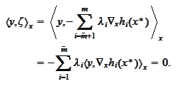
In the condition 1 of the definition ( Pseudonormality ) the LHS MATH is a vector of components of the gradient $\nabla_{x}$ . The scalar product applies to $i$ and $j$ indexes of MATH and MATH . We apply the scalar product with respect to components of the gradient $\nabla_{x}$ and write the following consequence of the condition 1: MATH Here we used that MATH for $X=\QTR{cal}{R}^{n}$ . We rearrange the terms as follows MATH Therefore, the $\lambda$ and $\mu$ as in the definition ( Pseudonormality ) cannot exist because the first sum MATH is zero by the condition MATH of the proposition and the second sum is negative by the condition MATH of the proposition and the condition 2 of the definition ( Pseudonormality ).

Proposition

(Constraint qualification 3). If $X=\QTR{cal}{R}^{n}$ , $x^{\ast}\in C$ , the functions MATH are affine and the functions MATH are concave then the vector $x^{\ast}$ is pseudonormal.

Proof

By the conditions on $h_{i}$ and $g_{i}$ we have MATH for any MATH . Therefore, for any $\lambda$ and $\mu$ MATH By the inclusion $x\in C$ , the first sum is zero and the second sum is non-positive. Hence, if $\lambda$ and $\mu$ satisfy the condition 1 of the definition ( Pseudonormality ): MATH then the condition 3 of the definition ( Pseudonormality ) must fail.

Proposition

(Constraint qualification 4). Let $X=\QTR{cal}{R}^{n}$ , $x^{\ast}\in C$ , the $x^{\ast}$ is pseudonormal for the set MATH

and for some $\bar{r}<r$ . Furthermore, there exists a MATH such that MATH

Proof

Note that MATH because if MATH then $\mu=0$ and the conditions 1,2,3 of the definition ( Pseudonormality ) are satisfied for the set $\bar{C}$ . The rest of the proof is a repetition of the proof of the proposition ( Constraint qualification 2 ).

Proposition

(Constraint qualification 5). Assume that the following conditions are satisfied.

1. The functions MATH , $i=\bar{m}+1,...,m$ are linear for some $\bar{m}\leq m$ .

2. The does not exists a MATH such that MATH and not all MATH are zero.

3. Let MATH Either MATH Interior MATH or $X$ is convex and MATH .

4. There exists a MATH such that MATH

Then the vector $x^{\ast}$ is pseudonormal.

Proof

We assume that all the conditions of the definition ( Pseudonormality ) hold and reach a contradiction.

We introduce the notation MATH According to the condition 4 of this proposition and condition 2 of the definition ( Pseudonormality ), there exists a MATH such that MATH The condition 1 of the definition ( Pseudonormality ) requires that MATH thus MATH Hence, we already proven the statement for the case MATH .

It remains to consider the case MATH under the assumption that the conditions 1,2,3 of of the definition ( Pseudonormality ) and the conditions 1,2,3,4 of this proposition are true and arrive to contradiction. By the assumption MATH , we have MATH and by condition 2 of the definition ( Pseudonormality ) we have MATH The condition 1 of the definition ( Pseudonormality ) implies MATH Hence, by the condition 2 of the proposition, all MATH are zero: MATH By the condition 3 there is a $y$ from the interior of MATH such that MATH Hence, MATH Hence, we have found a point MATH and an interior point $y$ of MATH such that MATH This is a contradiction. For an interior point of a cone MATH we must have MATH


Notation. Index. Contents.


Copyright 2007