n the previous section
(
Remark on stability of
financial problems
) we pointed out the boundary difficulty when setting up
a finite difference problem in financial applications. There is at least one
class of problems when such difficulty is particularly dire. Consider the
following problem (Asian option).
We wish to evaluate the
expectation
 where the processes
 and
and
 are given by the
SDEs
 and the function
 is a given final payoff. The
 is the
integral
 Note that the straightforward
Backward
Kolmogorov's equation
for this problem has the
form

|
|
(Asian PDE)
|
The term
 is large on the lattice boundary because the
 is large. Hence, the loss of normality would be amplified on every step.
Consequently, there is no hope that straightforward discretization of this
equation would be stable.
The equation
 is well behaved. We would like to find
representation
 at least locally in time so that we could safely make one step of the finite
difference scheme. We now proceed to derive the form of such
 .
.
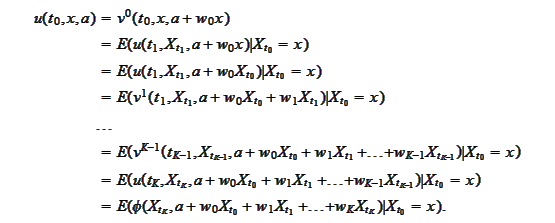
Note, that the function
 has the following
properties
 The second property is obvious. The first property is the consequence of the
(
Chain_rule
). These properties are also sufficient:
if
 has both of these then it solves the original problem.
Indeed,

Suppose we already calculated the solution
 at the time step
 and would like to derive the solution at the time
 .
This is our calculation scheme:
1. We set the final condition for
 at
at


2. We calculate the
 at
at
 according
to

3. We set
 We seek
 that provides the
property
 for all
 .
.
According to our calculation
procedure
 Note that the function
 satisfies the
condition
 for all
 because its defining
equation
 is the backward Kolmogorov's equation for the
problem
 Hence, it suffices to choose
 according
to
 Under such choice the expressions
 and
and
 have the same third argument.
Consequently,
 and
and
 We recall that by definition of

 Hence,

Normally, one would have to make sense of this procedure in the limit
 .
We are not going to do it. The process
 was introduced through an
SDE
 because the such SDE allows to write a two-dimensional PDE
(
Asian PDE
) for the function
 with subsequent transformation into finite difference scheme. We just
discovered that we do not need the (
Asian PDE
). In
financial applications the
 is a finite sum. The contract determines some set of times
 and set of weights
 .
The contract's payoff depends
on

We proceed to verify the validity of the above summary directly.
We
have

|