The
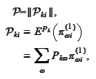
 is matrix multiplication. The notation
 is k-th component.
Definition
Given the market structure
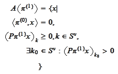
 the assumption of "no acceptable opportunities" is the requirement that the
set
 is empty. Note the absence of stress measures in the present definition (see
the last remark).
We are going to drop the stress measures from further considerations of this
chapter.
Notation
We introduce the following
notation


Hence,

Condition
(Basic coherence condition) We always
assume the
following:

Proposition
(Basic existence of
incomplete market pricing) There are no acceptable opportunities iff there
exists a pricing vector.
In other words
 iff there exists a vector
 s.t.
s.t.

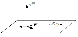
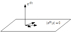
We explain the geometrical meaning of the proposition
(
Basic existence of
incomplete market pricing
) using the pictures
(
Incomplete Market
1
),(
Incomplete Market 2
).

|
Incomplete Market 1
|

|
Incomplete Market 2
|
If the projections of vectors
 on the plane
 are pointing in all directions then
 may be replicated by a positive linear combination of
 .
Otherwise, if the projections of
 are in the same half-plane with respect to any subdivision to half-planes in
 then such replication is not possible because then
 would have a non-zero projection on the plane.
It is now clear why we need the condition
(
Basic coherence condition
): If all
the
 lie in the plane then the replication is never possible.
Note that the vector
 is defined as a normal vector to some separating hyperplane. Set
 and consider the consequence of
 :
:

If we assume existence of a riskless asset then there is no choice but to
conclude
 .
Hence, the
 represents some convex combination of the original measures and the
equality
 means that
 is a risk neutral measure.
Definition
Given the set of available instruments
 we introduce the set of risk neutral probability
measures:

Corollary
If there are no acceptable
opportunities and there is a riskless asset
then

Here
 refers to the convex hull across various ways to model the market (across the
index
 ).
).
Proof
Even though the corollary above clearly follows from considerations of the
present section, such considerations are not easily extensible to more complex
situations. Hence, we give a more generic proof.
For any portfolio
 with the property
 we introduce the
set
 Clearly, by assumption of no acceptable
opportunities
 The next task is to prove
that
 We argue by contradiction. Assume
 and
introduce
 By the assumption
 we have
 By the theorem (
Separating
hyperplane theorem
) there exists
 s.t.
s.t.
 From the latter inequality we derive that
 .
Then from the former inequality we
conclude
 But
But
 is another portfolio with the property
 .
Hence, we arrived to contradiction with the assumption of no acceptable
opportunities. We conclude that any finite intersection
 is non empty.
We next
want to prove that the intersection
 is not empty for any countable collection of
 .
We introduce the linear
subspace
 The
The
 may be empty. Any x s.t.
 may be represented as a
sum
 where the
 and the y has the property
 Also,
Also,
 Hence, we will restrict further proof to
 only (switch to the orthogonal complement of
 ).
For
 the set
 always has an interior. Let
 be the Lebesgue measure acting in the space of
 :
:
 .
By the structure of
 the mapping
 is continuous with respect to y. We choose some
sequence
 where
where
 is the unit ball. By taking a subsequence we
have
 for some
 .
We
have
 Since
Since
 always has an interior we also
have
 By taking further subsequence and using continuity of
 we
have
 where we use the notation
 for the difference of sets. Note, that
 has properties of distance between sets. Hence,
 cannot converge to zero (because
 and
and
 are
are
 small
and
 is at least as large as
 ).
Consequently,
 cannot converge to zero. Hence, we proved that
 is not empty for any countable collection
 .
.
To see
that the same statement holds for any collection
 we note that there exists a countable everywhere dense set
 on
on
 and
and
 is continuous. Hence, any
 is infinitely close to some point
 and we can always
have
 for however small
 .
Since
 we
conclude

It
remains to note that the structure of the set
 is such that the result extends from
 to general
 .
.
|