e continue
derivations of the sections
(
Review
of variational inequalities in maximization case
) and
(
Penalized
problem for mean reverting equation
). We are considering an equation of
the problem (
Penalized mean
reverting
problem
):

The penalty term is non-linear. We will treat it as equation's RHS. We will be
manipulating
 and time step
 to keep
 small.
We replace the term
 with
with
 :
:

 where
where
 is some collection of functions
 with increasing span when increasing
 .
We will call
 "probing functions". The set
 is selection of probing functions, to be discussed later. We discussed at the
end of the section
(
Impossibility of
backward induction
) that
1. It is not possible to replace the scalar product
 with a projection on a range of functions.
2. There is no need to use a sophisticated collection of probing functions.
This is not a step back from wavelet framework because we make no attempt to
project on span of probing functions.
We drop the scale index
 from
notation:

The functions
 and
and
 are given by decomposition
 and
and
 :
:
 for a known basis
 and some index selection
 .
Hence,

 where the indexes
 are added to the index selection
 to point out that these selections may be different. The scalar products
 are independent of market data and contract parameters and may be
precalculated. The memory requirements for storing such data do not increase
in multidimensional case because we use tensor product to construct bases.
For calculation purposes we note
that
 where
where
 ,
,
 are Gram
matrices
 and operation
 is applied to a column component-wise.
Finally ,we remark on inserting the penalty term into the discontinuous
Galerkin procedure. We use the summary
(
Reduction
to system of linear algebraic equations for q=1
). We
insert
 to maintain correct sign relationship between the penalty term and the time
derivative.
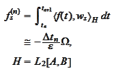
Then
 where
where
 is some discretization of the integral
 .
The summary
(
Summary for mean
reverting equation in case q=1
) applies with the
substitution
 Based on the matrix
 of the summary
(
Summary for mean
reverting equation in case q=1
) we apply the summary
(
Summary
for Black equation in case q=1, inverted matrix
) to calculate the matrix
 that
transforms

|
|
(Evolution with penalty term)
|
The following issues need resolution:
1. Selection of the probing functions
 .
.
2. Time-discretization
 of the
integral

3. Choosing between implicit and explicit formulations of
 .
.
4. Consequences of discontinuity
 within the definition of
 .
.
|