e
continue research of the previous section. The procedure has several problems:
1. For weak penalty term (high
 )
the procedure takes several time steps to converge to
 .
For strong penalty term (low
 )
it overshoots at the spacial boundaries of
 ,
taking the solution far beyond desired minimal installation at
 .
.
2. It picks up and accumulates discrepancy from correct solution while
converging into
 .
.
3. Boundary probing functions introduce discrepancy beyond
 area.
area.
Therefore, we propose to stop advancement in time until we iteratively and
minimalistically converge into
 using collections of internal probing functions of increasing precision.
Without time increment the evolution
 looks like
this:
 where the vector
 is input parameter,
 is a control parameter at our disposal,
 is a well conditioned matrix and
 has the
form
 for some wavelet basis
 and selection of probing functions
 .
We exploit the freedom of selection of probing functions by inserting control
parameters
 :
:
 Furthermore, we place probing functions conservatively within the area
 to make sure that no support of any
 intersects with
 .
The precision loss that comes from such requirement may be mitigated by
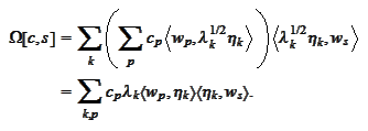
increasing scale of the probing functions. The penalty function
 now takes the
form
 We introduce the
notations
 then
then

 Let
Let
 The control parameters
 are optimized to
achieve
 with
constraints

We perform elementary
transformations:
 and arrive to the
problem
 This is a quadratic optimization problem with linear constraints. To make this
evident, we transform the problem to canonical
form:
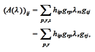
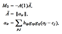
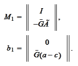
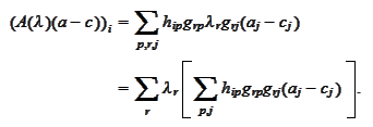 The problem takes the
form
 where
where

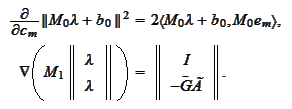
 The gradients for the problem
are
|