his section documents
generic and unsuccessful attempt to use backward induction, introduced in the
sections (
Backward induction
) and
(
Stochastic optimal control
)
in combination with finite element technique and a wavelet basis.
We are considering an equation of the problem
(
Penalized mean reverting
problem
):

Whatever discretization of the penalty
term
 we choose to consider, we would aim to correct
 into the
area
 after few, preferably one, time step. Why not do it directly? Indeed, we start
from a final payoff that satisfies
 .
Thus, penalty term would be zero. We make one step of penalty-free evolution,
apply some kind of a procedure that corrects the solution to
 and then do the same again.
We state with better precision what we intend to accomplish.
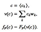
We have a solution
 given by a linear combination of a wavelet basis functions
 :
:
 We have another collection of non-negative valued functions
 with the same approximating
power:
 but without well conditioned Gram matrix
and

We introduce the
functionals
 and
notations
 The
The
 are linear functionals
 and their action is easily
computable:
 We would like to find a procedure for
modification
 with two requirements for all
 :
:
 Let
Let

 Altogether there are
 requirements and
 variables
 .
The requirement
 must be satisfied strictly because this is the area of primary interest: area
of no exercise. We know that this is possible because the
 satisfies
 .
For each
 ,
the equality
 is a hyperplane and
 taken for all
 is an intersection of hyperplanes. Since there are more requirements then
variables, existence of intersection is likely to be numerically unstable.
Therefore, we switch to the following
problem
 where
where
 is a parameter dictating strictness of
 :
:
 and
and
 are the scale-dependent factors we intend to manipulate for better stability.
The penalty term
 is
introduced for regularization.
The function
 has the
form
 where
where
 is an
is an
 matrix
 and
and

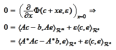
We proceed to calculate the minimum. Let
 be any non-zero vector and
 is a small positive real number,
then

 where the last equality holds at the minimum
 for any
 .
Therefore,
 is recovered by
solving
 The
limit
 is called "Moore-Penrose pseudoinverse". Calculation of
 is a well developed area. We
conclude

The numerical experiment is implemented in the script soBackInd.py located in
the directory OTSProjects/python/wavelets2. The procedure is unstable. The
parameters
 and
and
 create wild difference in results.
We offer the following intuition about sources of instability. We need to have
non-negative valued functions
 with the same approximating
power:
 The only way to accomplish this within wavelet framework and in a situation of
adaptive multiscaled basis is to take
 -based
scaling functions
 as the collection
 .
Those are the only non-negative functions in the framework. Functions
 only have the same approximating power if several of them are used with
consecutive indexes. Multiscaling feature means that we take
 -ranges
of
 for several
 .
But then the entire collection would be linearly dependent, because by
construction of
 ,
,
 and this is one source of the instability.
Using single scale
 collection of
 almost removes instability but lacks precision. If we use fine scale
 collection of
 then we defeat the purpose of using wavelets: we get a large poorly
conditioned matrix
 .
.
Another source of instability is the operation
 .
We already noted that
 have good approximating properties when taken together. Here, we take a single
scalar product. This is as good (or as bad) as taking scalar product with a
hut function. If we revert to some simple family of
 ,
such as hut functions, then we get a large
 .
.
Finally, we cannot replace a single scalar product operation
 with a projection on a range of
 because we would be unable to take the maximum
 component-wise.
Naturally, in one dimensional situation, one can simply take
 directly. Indeed, both
 and
and
 are piecewise polynomial functions. There are two problems with this approach:
1. We need to recombine decompositions
 into piecewise polynomial functions, take maximum and decompose again.
2. Such procedure, although already expensive, has no effective extension in
multidimensional case.
In the following sections we present a procedure that does not involve taking
maximum and extends smoothly into multiple dimensions.
|