e are
operating with the motivation of the section
(
Markovian projection
). The
reference for this section is
[Antonov2006]
. The goal
is to approximate the process
 of the
form
 using the process
 of the
form
 Here the
 is some generic process (existence/uniqueness restrictions apply),
 and
and
 are deterministic functions. This corresponds to restricting our attention to
minimization among the class of linear functions. We
seek
 where the
 refers to the scalar product in two dimensions. Hence, we will be evaluating
variations with respect to
 and
and
 and equating them to zero. We seek
 and
and
 such
that

 where the
 and
and
 are any smooth deterministic functions. We proceed with calculation of the
derivatives:

 where we introduced the notation
 .
Hence, the functions
 and
and
 are solved from the two equations
 and
and
 in terms of the expectations
 ,
,
 ,
,
 .
The
.
The
 is significantly easier to calculate because
 may be represented as a solution of a system of ODEs. We will see examples of
such technique immediately below and in few following sections. Moreover, we
are already operating in the approximation mode, hence we may expand in series
of the volatility scale (assuming that the general magnitude of volatility is
much less then 1). We establish that
 is of magnitude
 :
:


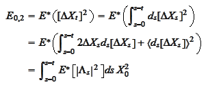
|
|
(Variance of target process)
|
and consider leading terms of the equations
 and
and
 :
:
 The leading terms of the second equation
are
 hence
hence

|
|
(MarkPr1 Sigma)
|
The leading terms of the first equation
are
 hence
hence

|
|
(MarkPr1 Beta)
|
Similarly, to (
Variance of target
process
) we apply
 operation under the expectation sign and produce an ODE problem for all the
interesting expectations.
|