ollowing sections (
Markovian
projection
) and
(
Markovian
projection on displaced diffusion
) we are developing a generic recipe for
approximation of the process
 given by the
SDE

|
|
(MarkPr TargetEquation)
|
with some adapted diffusion process
 .
We will be using Heston-type processes as the class of approximating
processes.
The reference for this section is
[Antonov2007]
.
In line with the section
(
Heston_equation_section
) we seek
approximation in the class of the stochastic processes given by the
equations

|
|
(Heston approximation)
|
for variety of deterministic functions
 .
The
.
The
 are standard Brownian motions. The
 refers to the difference
 .
The analytical tractability of the equations
(
Heston approximation
) was considered in
the sections (
Heston equation
) and
(
Displaced diffusion
).
Note that we may write the equation (
MarkPr
TargetEquation
) in the equivalent
form

|
|
(MarkPr TargetEquations 2)
|
for some diffusion processes
 ,
,
 ,
,
 and
and
 To see that the equations (
MarkPr
TargetEquations 2
) are equivalent to
(
MarkPr TargetEquation
) observe that we
may introduce the process
 and claim that it a diffusion because
 is assumed to be a diffusion. Consequently, we introduce the diffusion
process
 The process
 have correlated and uncorrelated components of the diffusion term, hence, we
have the sum
 for some processes
 ,
,
 .
Finally,
 is positive, hence the multiplication by
 does not restrict the generality. The motivation behind such transformation is
the aim to present the target process
 in the form similar to the form of the approximating process
 .
.
We will be applying the Gyongy's result
(
Multidimensional Gyongy lemma
),
hence, we put the target and approximating processes in the matrix form. We
seek to approximate
 with
with
 given by the
SDEs

 Note, that according to the lemma
(
Multidimensional Gyongy lemma
)
a general 2-dimensional
process
 may be replicated by the local volatility
process
 with the functions
 ,
,
 given by the
relationships
 We note that in our setting
 and
and
 .
Following motivations of the previous section
(
Markovian projection section
)
the functions
 ,
,
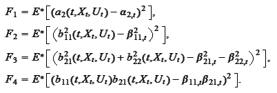
 minimize the following
functionals:
 We substitute the expressions for
 :
:
 and simplify
to

The rest of the calculation is a straightforward extension of the previous
section
(
Markovian
projection on displaced diffusion
). We calculate the variations of the
functional


 We minimize the functional
 :
:
 We calculate variations of the functional
 :
:

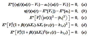
 We summarize the results of
minimization:
 The functions
 are defined by (a) and (b). The absolute values
 is defined by (c). The
 and
and
 are defined by (d) and (e). The expectations are calculated by techniques
outlined in the previous two sections.
|