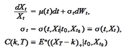
uppose a stock
 follows the
SDE

 in the risk neutral world. The
 is a deterministic function of time. The
 is the moment of observation. We aim to express the volatility
 as a function of
 and its derivatives with respect to strike.
We use the
representation
 in terms of distribution density
 We calculate the
 -derivative
 and substitute the equation
(
Forward_Kolmogorov
):

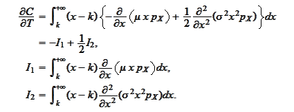
We evaluate each integral via integration by parts and with help of results
(
Distribution density via Call
).

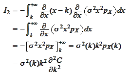
Summary
(Differentiating
call with respect to maturity
1)Assume
 then
then

We now switch to a process of the
form

 where the function
 is still given by
 Thus we cannot simply do a
 -change
of variables to reduce to the previous case. We repeat our
calculations.

 The equation (
Forward_Kolmogorov
) now has
the
form

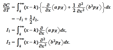 We integrate by parts and use the formulas
(
Distribution density via
Call
):

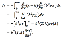
Summary
(Differentiating
call with respect to maturity 2)
Assume
 then
then

|