e are considering a debt structure
with payment dates

 We introduce the following
notation

|
|
(Libor2)
|
We introduce the probability measure
 associated with the price
 taken as a numeraire,
 .
The
.
The
 is an increment of the
 th
standard Brownian motion under the
 .
It is the assumption of the model that the process
 is
lognormal
 under
under
 for any
 ,
where the
 are some deterministic functions. The increment
 ,
,
 ,
has a drift under

 The calculation of
 is our next task. According to the formula
(
Change of drift recipe
1
)

By the definition (
Libor
definition
),
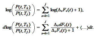
 Hence, for
 ,
,

 We use the formula
(
Change_of_drift_recipe_1
),
 Therefore

 where the
 are correlations and
 are volatilities of the forward
rates
 Similarly, for
 ,
,

LIBOR market model introduces a curve-dependent drift. Hence, it has a state
variable (=description of filtration) of high dimensionality.
|