he Heston equations are of the affine type. Hence, we proceed as discussed in
the section (
section about Affine
equation
).
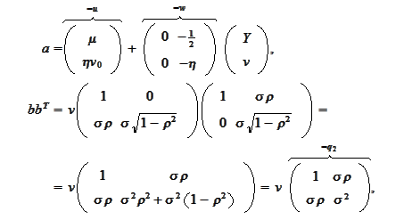
We transform the equations to the
 -form (
Affine equation
). Let
 ,
,

 hence
hence
 In
particular,
 According to the summary (
Affine
characteristic function 1
)-(
Affine
boundary conditions
) the
function
 is given by the
expression
 where the functions
 and
and
 must satisfy the following system of
ODEs:


 We transform the above
relationships:
 The
The
 are to satisfy the final
conditions:
 The next task is to solve the
equation
 We introduce the convenience
notation
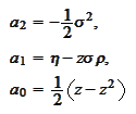 and
write
 We perform the change of the unknown
function
 as
follows
 We perform the
transformation
 as follows:
 In
addition,
 Hence,
 and,
consequently,
 We arrived to a linear equation. We look for solutions of the
form
 It suffices to
have
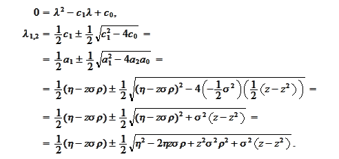 We mean to integrate over
 because this is the argument of the characteristic function and we want to
take the inverse Fourier or Laplace transform. Note that when
 the expression under the square root is positive. For large
 it is negative. Hence, we would rather change
 for real
 .
Then the square root is never zero. Indeed, the real part would be
 ,
where the correlation
 is not greater then 1.
We perform the backward
substitutions
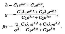 We introduce the quantity
 according to the relationship
 and transform the expression for

 to emphasize that the requirement
 uniquely identifies the
 .
.
We now consider the equation for
 :
:
 where the
 is a constant and the
 has just been
calculated:
 We
have
 hence
hence
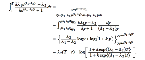
 It remains to evaluate the
integral
 Since
Since
 satisfies the final
condition
 we
have

|