imilarly to the
section (
Localization
), we are going to
calculate the interval
![$\left[ A,B\right] $](graphics/notesCF__2__1437.gif) .
.
In the section (
Mean reverting
equation
) we calculated that the
SDE
 may be integrated
into
 We
continue
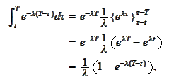
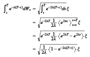
 The integrals
evaluate

 for a standard normal random variable
 .
We put the results
together:

|
|
(Mean reverting solution)
|
where we introduced the convenience notations
 and
and
 ,
,
 ,
,

Based on a precision
 ,
,
 ,
we would like to find two numbers
 and
and
 such
that
 We
calculate

 Let
Let
 be a number
s.t.
 then
then
 and
and

The process
 is connected to
 of the section
(
Solving
one dimensional mean reverting equation
) by the
relationship

|
|
(Exponential change)
|
 We aim to set the interval
![$\left[ A,B\right] $](graphics/notesCF__2__1464.gif) according
to
according
to
 However, we still need to make two more modifications:
1. We need to adapt
 to the binary structure of our mesh. Similar argument was already made in the
section (
Localization
).
2. We want to make
![$\left[ A,B\right] $](graphics/notesCF__2__1467.gif) time independent for smaller difference
time independent for smaller difference
 .
.
To achieve the goal 2 we
set

 We choose
 conservatively wider to preserve precision. Adaptive basis selection is a
compensating procedure that preserves efficiency.
For the goal 1, we choose a scale parameter
 and
and

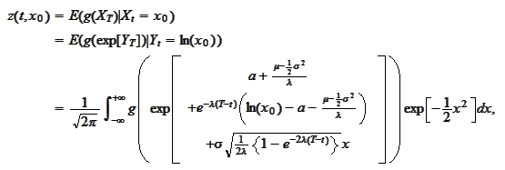
The following is a consequence of the formulas
(
Mean reverting solution
) and
(
Exponential
change
):

|
|
(Analytical solution for mean reverting equation)
|

|