he
scripts basis3.py, basis3a.py, project.py in the directory
OTSProjects/wavelets2 contain the following derivations.
We would like to obtain a decomposition for a
function
 with respect to a wavelet basis adapted to the interval
 .
.
We start from results of the procedure
(
Calculation
of approximation spaces in one dimension II.
) We have the sets of
functions
 We adapt these functions to the interval
 by applying the operation
 to each
function:
 normalize them to
 .
This is done in basis3.py and basis3a.py.
In the script project.py we initially
calculate
 where the
 is the minimal scale that satisfies the condition
(
Sufficiently fine scale 2
) and the
projection is taken in
 .
.
We form the
set
 for some fixed
 .
Then we repeatedly
do
 until
until
 reaches a given number.
This experiment yields the following conclusions:
1. Approximation is significantly better then anything that may be obtained by
classical finite elements or low order wavelets.
2. Floating point errors break procedure for reasonably large
 if we use the Poly class. We successfully remove the difficulty using the
localized piecewise polynomial representation of the functions
 covered in the section
(
Manipulation
of localized piecewise polynomial functions
).
3. Accelerated version of the procedure involves taking several functions of
the same scale on the
step
 The number of functions decreases with scale and increases with required
precision or
 .
Another way to accelerate the procedure is to gradually increase the set
 based on results of previous steps.
One does not need to calculate wavelet decomposition at every evaluation
because of scaling and translation properties of the wavelet basis. The
decomposition may assembled almost instantly and with perfect precision from
precalculated data.

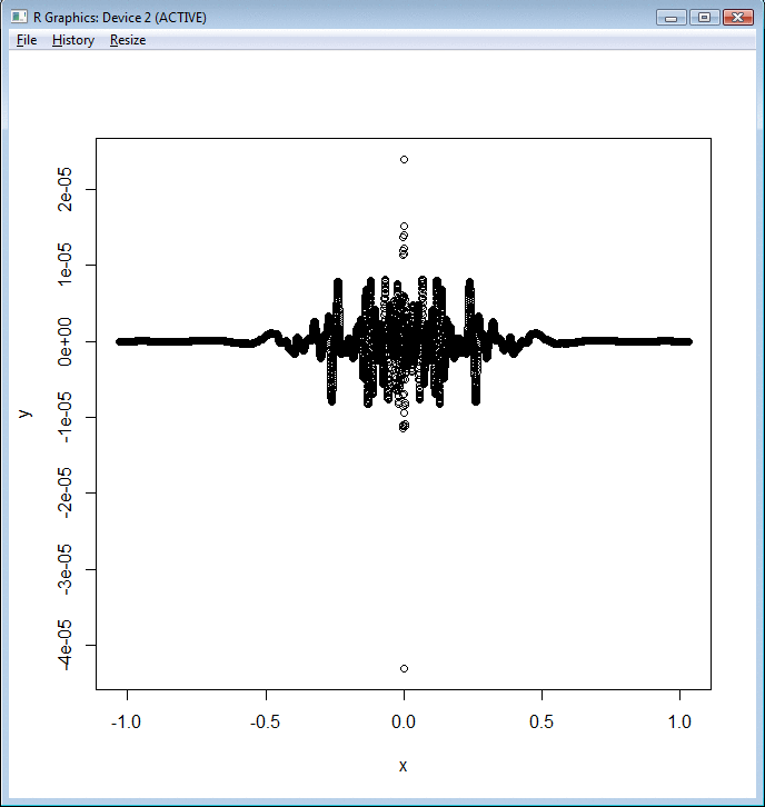
Plot of
 for
for
 executed using LPoly.
|
The script dproject.py contains a similar experiment performed in
 -space.
Note that the resulting recipe is opposite to the recipe of the section
(
Adaptive approximation
).
Indeed, the wavelet basis approximates perfectly the linear part of the
function
 and has difficulty around the singularity. However, it is around the
singularity where the function
 has the smallest variation.
|