e introduce the remainder
Definition
(Remainder of averaged
Taylor
polynomial)

According to the proposition
(
Properties of averaged
Taylor polynomial
)-2 and formula
(
Mollifier for a ball 2
), for a
function
 we
have
 We introduce the function
 :
:
 According to the proposition
(
Integral form of Taylor
decomposition
),
 and
and
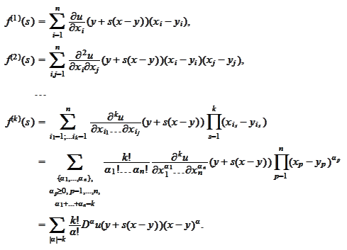 Consequently,
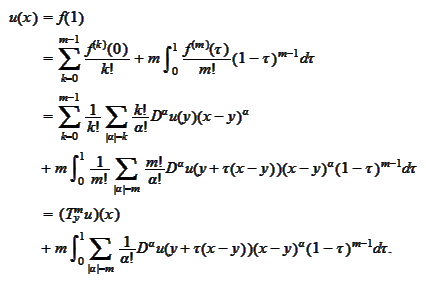
We continue calculation of
 :
:
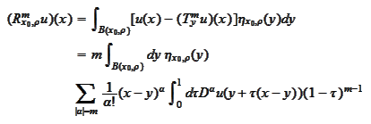 Our goal is to transform the integral to the form
 .We
make the change
 in the
 -integral,
 ,
,
 ,
,
 We aim to make a change of variables
 where
where
 .
Hence, we change the order of integration (see
(
Fubini
theorem
))
 and proceed with the change
 ,
,
 ,
,
 ,
,

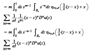 We would like to put result in the form
 ,
hence, we reverse the order of integration again. The set of integration is
 Note that the line
 for a fixed
 connects
 with a point
 in
in
 .
Thus, the
 -plane
projection of the set
 is the convex hull of
 and
and
 :
:
 Let
Let
 be the section of
 with a plane
 :
:
 We continue the
calculation:
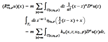 where the functions
 are given
by
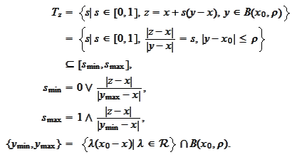
 We estimate (see the figure
(
Estimation of averaged
Taylor
polynomial
))
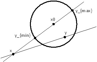
|
Estimation of averaged Taylor
polynomial
|
Thus
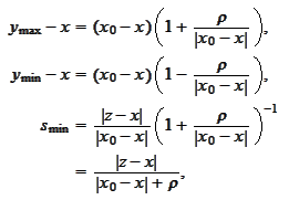 We
state
 and estimate the
 :
:
 Note that
 ,
,
 hence
hence
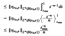 By the formulas (
Mollifier for a ball
1
),(
Mollifier for a ball 2
) and the
definition (
Standard mollifier
definition
)-2
 where the
 depends on
 ,
so we drop
 and substitute for
 :
:
 We summarize our findings in the following proposition.
|