his section documents a negative result.
We would like to construct a preconditioner via exact inversion of the Black
PDE.
In the section
(
Asymptotic
expansion for Black equation
) we calculated solution for Black equation.
Let
 be the solution of the
problem
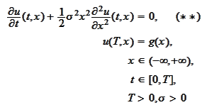 for integrable function
 then
then
 We would like to put the expression into the
form
 for some kernel
 .
We introduce the
notation
 then
then
 We make the
change

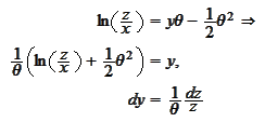 then
then


We introduce the projections of
 on some basis
 and index set
 .
We
approximate
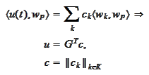
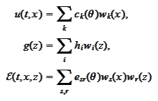 then we apply the operation
 to the equation
 and
obtain
 Thus
Thus
 where the
 are
columns
 and
and
 are
matrixes

Note
that
 and
and
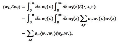
 It follows from

 or
or
 We intend to use (some approximation of)
 as a preconditioner. We need some way to evaluate the integrals
 perhaps with relaxed precision. The simplest road is to use crudification
operator to simplify piecewise polynomial representations of the basis
 ,
make square of the number of pieces below 256 and then employ Cuda.
The functions
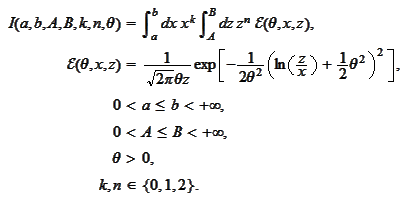
 are piecewise quadratic polynomials. Our next task is to calculate expressions
for the
integrals
 We calculate the
 -integral:
 We make the change

 We complete the
square:

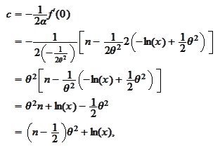
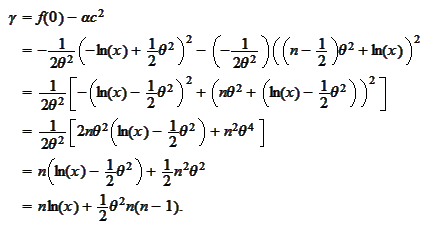 Thus
Thus
 We make the
change


We cannot proceed with explicit evaluation of the
 -integral
from this point. Hence, we perform a linear approximation of the function
 on the interval of interest
 :
:

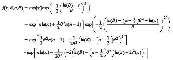
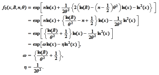
 Make the change
 then
then
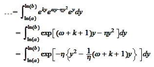 We complete the
square:
 and do linear
approximation

We put our results
together.


Due to lack of absolute precision and the number of required numerical
operations this approach does not offer improvement over combined application
of recipes of the sections
(
Diagonal preconditioner
) and
(
Reduction to well
conditioned form
). The author did not do a numerical experiment or
verification of the above summary.
|