he following is the program of our
actions:
 We start from the uniform on
![$[0,1]$](graphics/notesCF__0__2352.gif) random variables
random variables
 and apply the Box-Muller procedure, described in the claim
(
Box-Muller procedure
). The step
 is a unitary linear transformation of the iid standard normal variables
 into a jointly normal variables
 .
The transformation
 produces two correlated uniform variables according to the
(
Sklar_theorem_2
). The transformation
 is the application of the (
Sklar_theorem_1
).
We spell out every step below.
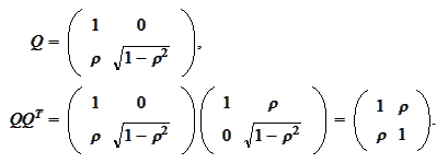
We choose the transformation
 ,
,
 to construct the
 with the following
properties
 We observe
that
 Hence, it suffices to chose
 according
to

The step
 is performed according to the idea behind the result
(
Sklar_theorem_2
). We note that the cumulative
standard normal distribution
 produces a uniform on [0,1] random variable
 from a standard normal variable
 according to the rule
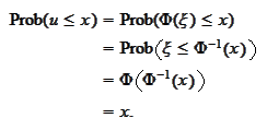
 Indeed, for such
 we calculate

We also introduce the function
 and uniform on [0,1] random variables
 :
:
 Hence,

For the final step
 we are given the cumulative distributions
 .
We simulate the variables
 and
and
 according to the
rules
 Such variables have marginal cumulative distributions
 and
and
 respectively. Their correlation is controlled by the parameter
 .
The joined distribution is given by the following
calculation:
 If
If
 is 0 then the
 splits into product and the
 are uncorrelated. Preservation of sign of correlation takes place.
|